CMEP: XBeach, a storm impact model for sandy beaches

Ben Phillips

National Oceanography Centre & University of Liverpool

benp@noc.ac.uk

Twitter: @btphillips94

Further information: https://xbeach.readthedocs.io/en/latest/user_manual.html

Introduction

XBeach is an open-source numerical model which is originally developed to simulate hydrodynamic and morphodynamic processes and impacts on sandy coasts with a domain size of kilometers and on the time scale of storms. It can be used to simulate wave run-up, beach erosion and sediment transport. Whilst capable of being run in two dimensions (i.e. longshore and cross-shore), here we will only be using a basic one-dimensional cross-shore setup. In this workshop, you will become familiar with how to setup and run a basic XBeach model, and how to use Python to plot wave run-up and changes in a beach profile during a storm.

Before the workshop

Please make sure you follow the steps below, to install the necessary software prior to the workshop.

We will be working with Windows only, as there are no pre-compiled XBeach executables for Linux or Mac systems. Please arrange access to a Windows system for this workshop (if you don't already have one).
Create two folders. Name one "XBeach" and the other "XBeach-data".
Download the XBeach model. We will be working with the Windows 2015 'Kingsday' version available here, extract all files into the "XBeach" folder.
In order to set-up XBeach and analyse model outputs, we will use Python. The easiest and safest way to install Python is by using Anaconda, which installs the most commonly used libraries, and easily allows the user to install additional ones when and if required. Please go to this link https://repo.anaconda.com/archive/Anaconda3-5.3.1-Windows-x86_64.exe and download Python 3.7 Windows 64-bit. It also installs Spyder, a MATLAB like Graphical User Interface, which you can use to load, edit and run Python scripts.
Please download the zip file containing the following required Python scripts and model data here, and extract them into your "XBeach-data" folder.
Download the workshop environment file by clicking here and save it into your XBeach-data folder
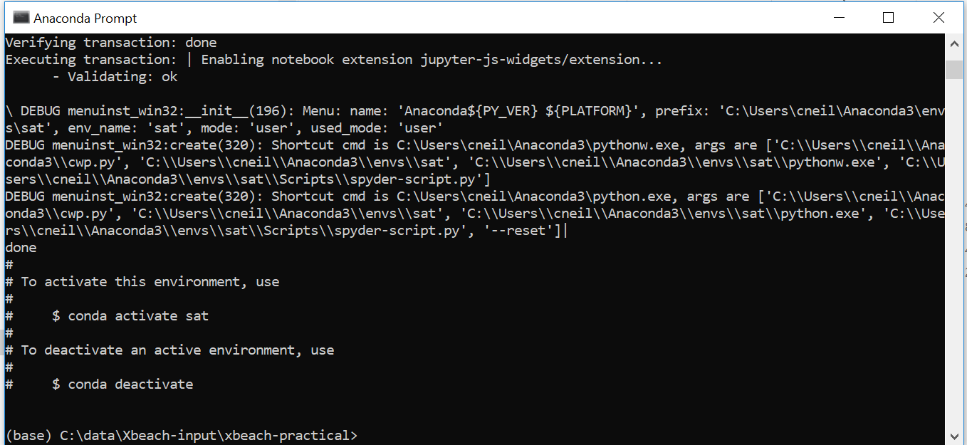
Once you have Python installed, open up Anaconda Prompt, navigate to your "XBeach-data" folder using the "cd" command and type on the command line: conda-env create -f workshop_environment.yml and press enter. Once this has finished installing, type on the command line: conda activate sat and press enter. Then type spyder and press enter -This gets everything ready for the XBeach and Python sessions, and will open a program called Spyder which we will be using later.

Python files:

aquadopp_setup_xbeach.py
awacs_setup_xbeach.py
models_setup_xbeach.py
plot_wave_runup.py
plot_storm_profile.py
cmep_xbeach.py
workshop_environment.yml

Model data:

WW3_Oct10.nc
nemo_Oct16_Nov16_2010.nc

Observational data:

SVG-Wave-Data-Jul-Oct2018.xlsx
Grand-Anse-Aquadopp.xlsx

Beach Profile data:

GAB_Beach_Profile.csv (Grenada)
Georgetown_Beach_Profile.csv (St Vincent)

Data requirements

Beach profile: A cross-shore profile extending from the beach to at least 10 m water depth.
Water level data: Time series provided by a model (e.g. NEMO) or from observations (tide gauge, AWACS buoy etc.).
Wave data: Time series of wave height and period provided by a model (e.g. WaveWatchIII) or by observations (e.g. an AWACS buoy).

Setting up a basic XBeach model

This section of the workshop provides single Python scripts to set-up the whole model, with files in the correct format. Also detailed are some slightly more complicated options which would also allow you to represent erosion of the beach, but ensuring that fixed structures remain non-erodible. Please read through the Beach profile, Waves, Water Levels and XBeach: Parameters file to familiarise yourself with the inputs, then attempt the exercises.

Beach Profile

In order to ensure the model runs smoothly, the profile we provide needs to extend down to at least 10 m water depth, or double the offshore wave height (whichever is greater). This is to ensure the offshore boundary is sufficiently deep to prevent waves breaking on the model boundary. If data does not extend this far, assume the remainder of profile is a simple linear slope based on a sensible value between the end of the profile and the offshore boundary. Here, we will take a basic beach profile (e.g. Figure 1) and by using some Python functions, convert it into suitable input for XBeach.

There are three files required, with one value for X,Y and Z for each point in the profile.

X: Cross-shore distance (m). Distance along the profile between the offshore boundary and the beach. This is referred to as the grid file

Y: Alongshore distance (m). As we are using a cross-section, each grid point will have a value of zero.

Z: Elevation (m). One value for each point. This is referred to as the bed file.

There are two main stages to this.

Ensuring you have a series of X and Y co-ordinates and corresponding elevations (Z), extending from at least 10 m water depth to the shore, or from further offshore under extreme wave conditions.
Putting these values into a Python script to ensure the grid has a sufficient number of points (a minimum of 25 per wavelength).

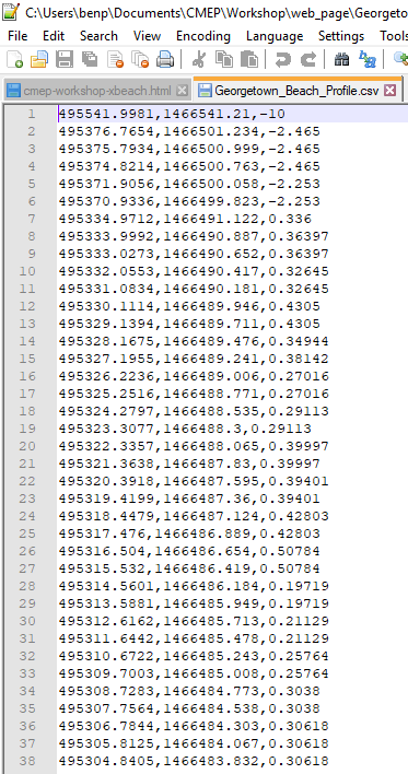
Open up the beach profile (St Vincent: Georgetown_Beach_Profile.csv or Grenada: GAB_Beach_Profile.csv) and have a look, the format is shown below:

X[sea],Y[sea],Z[sea]

X[1],Y[1],Z[1]

X[land],Y[land],Z[land]

Each line contains X and Y co-ordinates, and the corresponding elevation, with values separated by commas. The file begins from the seawards end of the profile (see image below for an example). The end of the profile can be extended automatically in the setup script based on the specified depth (Dsf) and Slope values, but the provided profiles are sufficient, so they do not need editing.

Adding non-erodible structures

When running with morphological evolution enabled, XBeach can output the changes in the beach profile throughout the storm event from erosion and/or sedimentation. But when doing this, we may need to represent fixed, non-erodible structures such as sea walls or cliffs in the profile. Fortunately these structures are fairly straight forward to represent in the model. The only requirement is an additional file which specifies either 0 (non-erodible) or 10 (erodible, 10 m of sediment available) for each grid point. By specifying the elevation of the bottom of a fixed structure, the model setup scripts will create this file automatically, ensuring only the beach can be eroded. Setting the CliffedBeach option to True inserts a non-erodible 10 m cliff at the end of the profile.

Waves

XBeach uses wave conditions on the offshore boundary and propagates them towards the shore. Lots of different options and settings exist, but here we will use the "non-hydrostatic" mode with a JONSWAP wave spectrum, which models the propagation and decay of individual waves. We will use a time series of significant wave heights and wave periods.

A basic waves file looks like this:

The first and second values in a row refer to wave height and wave period, respectively. The 3600 refers to the frequency of the measurements (in seconds). So here we have two hours of wave conditions. All the other values are default settings, there is no need to alter these.

Water levels

XBeach can take a time series of water level data, allowing the model represent storm surges experienced during hurricanes. Below is an example of a typical tide file, where we have hourly tide gauge data:

where time (in seconds) is in the first column, and the water elevation is in the second, seperated by a space.

XBeach: Parameters file

The model is controlled by a single parameters file which is always called 'params.txt' (the model will not recognise other filenames). This file contains the settings for the model as well as defines the grid, wave and tide conditions. Whilst XBeach contains a lot of settings, it is sensible to allow the model to take the default settings for most parameters, minimising the number of parameters that you set manually. Below is a basic parameters file with the very minimum you need to specify in order to run XBeach to output wave run-up on a fixed beach profile along with an explanation.

Underneath is a parameters file for a slightly more complicated set-up. Here, the parameters file is set so that XBeach also models sediment transport and the changes in the morphology of the beach profile, but keeps the sea wall or cliff fixed. This achieved by setting ErosionEnabled in the Python script to True, and setting StructureElevation to the height of the toe of the sea wall or cliff (or leave as None if the profile is just a beach).

As you can see most of the file is unchanged apart from:

Morphology and sedtrans are now set to 1
The addition of 'global output', saving values for each grid point over time, rather than just a single wave run-up value.
Two extra lines are required to add the sea wall or cliff. 'struct = 1' and 'ne_layer = ne_layer.dep', which specifies the files containing the 0 and 10 values described in the "Adding non-erodible structures section".

Physical processes:

morphology = 0 (fixed profile) or morphology = 1 (erodible profile)
sedtrans = 0 (disable sediment transport) or sedtrans = 1 (enable sediment transport)
Note: the default setting enables both, so here we are disabling both

nonh = 1 (resolves each individual wave)

Grid parameters:

xfile = file containing the cross-shore (x) co-ordinates for each grid point. The setup script calls this file x.grd
yfile = file containing the alongshore (y) co-ordinates for each grid point. The setup script calls this file y.grd
nx = the number of grid points -1
ny = always 0
depfile = the file containing the elevation of each grid point. The setup script calls this file bed.dep

Model time:

tstop = length of time to run the model for (seconds)

Tide boundary conditions:

zs0file = file containing a time series of water level. The setup script calls this file tide.txt

Wave boundary conditions:


bcfile = file containing a time series of wave heights and periods

Output variables:

outputformat = netcdf (recommended as it outputs 1 single file)
tintp   = 0.5 (save interval in seconds for outputting wave run-up)
Note: The smaller the save interval, the larger the file size!

Global Variables:

Global variables refer to variables where the model saves a value for each grid point on the beach profile. This is particularly useful if you want to simulate beach erosion, but is not required just for wave run-up. nglobalvar = the number of different variables you wish to save. Make sure they start on the line directly underneath. For example:

nglobalvar = 1
zb (bed level - allows us to plot erosion)

tintg = 60 (save an output every 60 seconds, again be wary of filesize)

There are lots and lots of different outputs from XBeach, but these ones are the most relevant for the workshop and the foreseeable future.

Run-up gauges:

nrugauge = 1
-1414.74712911851 0
The values above refer to the X & Y co-ordinates of the offshore boundary. Hence the second value is always zero, the first value is equal to the first value in x.grd

Exercises

Now you know the inputs required by XBeach, have a go at setting it up using the scripts provided. Work through the following two sections, and set the model up using the provided scripts, first with the observational AQUADOPP data, and then the modelled data. Switch back to Spyder, which should already be open. Spyder is a program which will allow you to load, edit and run Python scripts, as shown below.

You can open and run scripts as shown in the left hand and middle red boxes
Make sure your working directory is set to your XBeach-data folder (see red box on right hand side)

Setting up XBeach from observational data

Grenada: Converting AQUADOPP data into XBeach input

Here, we will be converting the AQUADOPP data from the Grand Anse deployment into XBeach input. Please open the spreadsheet containing the AQUADOPP data (Grand-Anse-Aquadopp.xlsx) which can be found in the downloaded zip folder.

What do we need from this file?

Basic information such as location, the depth it was deployed at, the height of the mounting sensor (WHR file tab)
The columns we need are: Hm0 = significant wave height (m), Tp = peak period (seconds), Mean pressure (decibars)

We know from the UK Hydrographic Office survey that the AQUADOPP was located in 8.5 m water depth, and that the mounting height is 0.5 m. Therefore the distance between the surface and the sensor is -8 m. We need to know this to able to convert the pressure data to a water level.

You need to provide a series of wave height (metres), wave period (seconds) and mean pressure (decibars) values for the period of time you want to run. You can produce this by copying the data from Excel into a seperate spreadsheet and saving it as a CSV (Comma separated value) file. Make sure you have a continuous time series. To start with, please do not select more than 2 values in order to reduce the length of time XBeach takes to run, and to allow you to plot the output.

Please ensure the file is in this format:

Hm0[start],Tp[start],Pressure[start]

Hm0[1],Tp[1],Pressure[1]

Hm0[end],Tp[end],Pressure[end]

A Python library containing functions to create the grid and the input files has been provided for this workshop and your further use. This file is called cmep_xbeach.py. Please ensure it is in your working directory.

The script you will edit and run to set-up the XBeach model is entitled aquadopp_setup_xbeach.py. Please ensure it is in your working directory, with the cmep_xbeach library, AQUADOPP and beach profile data.

Before attempting to run the script, please ensure you have:

Beach profile data: In a X,Y,Z format starting at the seawards end of the beach profile and moving landwards
AQUADOPP data: In a Hs,Tp,Pressure time series format, as shown above. This script assumes that the unit of pressure is decibars.

# -*- coding: utf-8 -*-

"""
Created on Fri Nov 23 10:27:15 2018
aquadopp_setup_xbeach.py
@author: benp

GRENADA exercise

This script will set-up a grid, waves, water levels and the parameters file for a basic XBeach simulation, using AQUADOPP
data from the Grand Anse Bay deployment as inputs. 
"""

#load libraries
import cmep_xbeach as xb
import matplotlib.pyplot as plt
plt.rc('font',size=20)

#Set filenames and settings for XBeach here

#AWAC settings
AWACSFile = 'aquadopp_data.csv' #Amend this to the filename containing your wave and pressure data
MeasurementFrequency = 3600 #Frequency of wave measurements (seconds)
AWACSDepth = -8.0 #difference between surface and sensor (m)

#beach profile settings
ProfileFile = 'GAB_Beach_Profile.csv'
ErosionEnabled = True #False to disable beach erosion. Change to True to enable beach erosion
StructureElevation = None #if running with erosion enabled, specify height of sea wall toe/cliff (if applicable)
CliffedBeach = False #Adds a non-erodible 10 m cliff at the end of the grid if set to true.
Dsf = None #offshore elevation to extend profile to, leave as None if ProfileFile extends to sufficient depth
Slope = None #slope at which to extend profile, leave as None if ProfileFile extends to sufficient depth

##### Please do not edit anything below here ####
XBeachRunTime,MinWL,MaxWL = xb.XBeachAquadoppSetup(AWACSFile,MeasurementFrequency,AWACSDepth)
XBX,XBY,XBZ,NE = xb.xbeach_grid_bed_setup(ProfileFile,Dsf,Slope,StructureElevation,ErosionEnabled,CliffedBeach)
xb.WriteParams(XBeachRunTime,(len(XBX)-1),XBX[0],StructureElevation,ErosionEnabled)
plt.plot(XBX,XBZ,'-xk',markersize=2.5)
plt.plot([XBX[0],XBX[-1]],[MaxWL,MaxWL],'b',label='Max. water level')
plt.plot([XBX[0],XBX[-1]],[MinWL,MinWL],'b--',label='Min. water level')
plt.xlabel('Cross-shore distance (m)')
plt.ylabel('Elevation (m)')
plt.legend(loc=4)

Setting up XBeach from observational data

St Vincent: Converting AWAC data into XBeach input

Here, we will be converting the AWAC data from the Georgetown deployment into XBeach input. Please open the spreadsheet containing the AWAC data (SVG-Wave-Data-Jul-Oct2018.xlsx) which can be found in the downloaded zip folder.

What do we need from this file?

Basic information such as location, the depth it was deployed at, the height of the mounting sensor (WHR file tab)
The columns we need are: Hm0 = significant wave height (m), Tp = peak period (seconds), Mean AST distance (m)

You need to provide a series of wave height (metres), wave period (seconds) and mean Acoustic Surface Tracking (AST, m) values for the period of time you want to run. You can produce this by copying the data from Excel into a seperate spreadsheet and saving it as a CSV (Comma separated value) file. Make sure you have a continuous series, as there are some errors and failed wave period measurements in the dataset. These are marked by error codes greater than zero in the spreadsheet. To start with, please do not select more than 2 values in order to reduce the length of time XBeach takes to run, and to allow you to plot the output.

Please ensure the file is in this format:

Hm0[start],Tp[start],Mean AST[start]

Hm0[1],Tp[1],Mean AST[1]

Hm0[end],Tp[end],Mean AST[end]

A Python library containing functions to create the grid and the input files has been provided for this workshop and your further use. This file is called cmep_xbeach.py. Please ensure it is in your working directory.

The script you will edit and run to set-up the XBeach model is entitled awacs_setup_xbeach.py. Please ensure it is in your working directory, with the cmep_xbeach library, AWACS and beach profile data.

Before attempting to run the script, please ensure you have:

Beach profile data: In a X,Y,Z format starting at the seawards end of the beach profile and moving landwards
AWACS data: In a Hs,Tp,AST time series format, as shown above.

# -*- coding: utf-8 -*-
%matplotlib qt
"""
Created on Fri Nov 23 10:27:15 2018
awacs_setup_xbeach.py
@author: benp

ST. VINCENT exercise

This script will set-up a grid, waves, water levels and the parameters file for a basic XBeach simulation, using AWAC buoy
data as inputs. 
"""

#load libraries
import cmep_xbeach as xb
import matplotlib.pyplot as plt
plt.rc('font',size=20)

#Set filenames and settings for XBeach here

#AWAC settings
AWACSFile = 'awacs_data.csv' #Amend this to the filename containing your wave and pressure data
MeasurementFrequency = 3600 #Frequency of wave measurements (seconds)
AWACSDepth = -9.5 #difference between surface and sensor (m)

#beach profile settings
ProfileFile = 'Georgetown_Beach_Profile.csv'
ErosionEnabled = False #False to disable beach erosion. Change to True to enable beach erosion
StructureElevation = None #if running with erosion enabled, specify height of sea wall toe/cliff (if applicable)
CliffedBeach = False
Dsf = None #offshore elevation to extend profile to, leave as None if ProfileFile extends to sufficient depth
Slope = None #slope at which to extend profile, leave as None if ProfileFile extends to sufficient depth

##### Please do not edit anything below here ####
XBeachRunTime,MinWL,MaxWL = xb.XBeachAWACSetup(AWACSFile,MeasurementFrequency,AWACSDepth)
XBX,XBY,XBZ,NE = xb.xbeach_grid_bed_setup(ProfileFile,Dsf,Slope,StructureElevation,ErosionEnabled,CliffedBeach)
xb.WriteParams(XBeachRunTime,(len(XBX)-1),XBX[0],StructureElevation,ErosionEnabled)
plt.plot(XBX,XBZ,'-xk',markersize=2.5)
plt.plot([XBX[0],XBX[-1]],[MaxWL,MaxWL],'b',label='Max. water level')
plt.plot([XBX[0],XBX[-1]],[MinWL,MinWL],'b--',label='Min. water level')
plt.xlabel('Cross-shore distance (m)')
plt.ylabel('Elevation (m)')
plt.legend(loc=4)

St. Vincent and Grenada: Setting up XBeach from WaveWatchIII and NEMO data

The script below will set-up XBeach using WaveWatchIII and NEMO model data for a given location and time period, Before attempting to run the script, please ensure you have:

Beach profile data: In a X,Y,Z format starting at the seawards end of the beach profile and moving landwards.
WaveWatchIII data: In the provided netCDF format.
NEMO data: In the provided netCDF format.
The cmep_xbeach.py and models_setup_xbeach.py files in your working directory.

The NEMO and WaveWatchIII files for the whole of the Caribbean are gigabytes large. In order to save file size and make the workshop run more smoothly, the files provided only covers the region around St Vincent and the Grenadines, and Grenada. Please therefore pick a point in this region otherwise your script will return an error.

Ensure you set the netCDF filenames, and the point for which you want to extract data. To start with, please do not choose more than 2 hours of data, in order to reduce the length of time XBeach takes to run, and to allow you to plot the output.

# -*- coding: utf-8 -*-

"""
Created on Fri Nov 23 10:27:15 2018
models_setup_xbeach.py
@author: benp

This script will set-up a grid, waves, water levels and the parameters file for a basic XBeach simulation, using NEMO
and WaveWatchIII netCDF files as inputs. 
"""

#load libraries
from netCDF4 import Dataset
import numpy as np
from datetime import datetime
import cmep_xbeach as xb
import matplotlib.pyplot as plt
plt.rc('font',size=20)

#WaveWatchIII netCDF file
WW3_file = 'WW3_Oct10.nc'

#NEMO netCDF file
NEMO_file = 'nemo_Oct16_Nov16_2010.nc'

#time at which you want to start and stop extracting data for XBeach
#format is dd/mm/yyyy HH:MM
StartTime = '18/10/2010 00:00' 
StopTime = '20/10/2010 12:00'

#The point for which you want data. For example here, the point at which the AWACS buoy was deployed
Latitude = 13.2683
Longitude = -61.1149

#beach profile settings
ProfileFile = 'idealised_profile.csv' #Grenada = GAB_profile.csv , St Vincent = GT_profile.csv
ErosionEnabled = True #False to disable beach erosion. Change to True to enable beach erosion
StructureElevation = None #if running with erosion enabled, specify height of sea wall toe (if applicable)
CliffedBeach = False
Dsf = None #offshore elevation to extend profile to, leave as None if ProfileFile extends to sufficient depth
Slope = None #slope at which to extend profile, leave as None if ProfileFile extends to sufficient depth

##### Please do not edit anything below here ####
XBeachRunTime,MinWL,MaxWL = xb.ExtractNemo(NEMO_file,StartTime,StopTime,Latitude,Longitude)
xb.ExtractWW3(WW3_file,StartTime,StopTime,Latitude,Longitude)
XBX,XBY,XBZ,NE = xb.xbeach_grid_bed_setup(ProfileFile,Dsf,Slope,StructureElevation,ErosionEnabled,CliffedBeach)
xb.WriteParams(XBeachRunTime,(len(XBX)-1),XBX[0],StructureElevation,ErosionEnabled)
plt.plot(XBX,XBZ,'-xk',markersize=2.5)
plt.plot([XBX[0],XBX[-1]],[MaxWL,MaxWL],'b',label='Max. water level')
plt.plot([XBX[0],XBX[-1]],[MinWL,MinWL],'b--',label='Min. water level')
plt.xlabel('Cross-shore distance (m)')
plt.ylabel('Elevation (m)')
plt.legend(loc=4)

Running XBeach

Now that you have run one of the two setup scripts, you have generated all the files you need to run XBeach. Below is a brief explanation of what each file contains, so you can double check that everything is correct, and copy the following files to your "XBeach" folder, which contains the executable.

x.grd - Cross-shore co-ordinates. File should begin at the offshore boundary, and increase towards the shore.
y.grd - Alongshore co-ordinates. Every value should be zero.
bed.dep - bed elevation. File should begin at the offshore boundary and increase towards the shore. Remember negative values are down.
tide.txt - tidal elevation. File should begin at zero and contain time and water level, in the first and second columns, respectively. The length of the file should equal the model run time
jonswap_table.txt - Wave conditions. The sum of the duration column should equal the model run time.
params.txt - Parameters file. Points XBeach towards the files specified above and sets all the options.
ne_layer.dep - Erodible/non-erodible points file. Tells XBeach whether a grid point is fixed (0) or not (10). Only required when running with ErosionEnabled = True.

If you are happy with everything, you can double click xbeach.exe and the model will then launch automatically. A separate window will open where you can monitor the progress, as shown below.

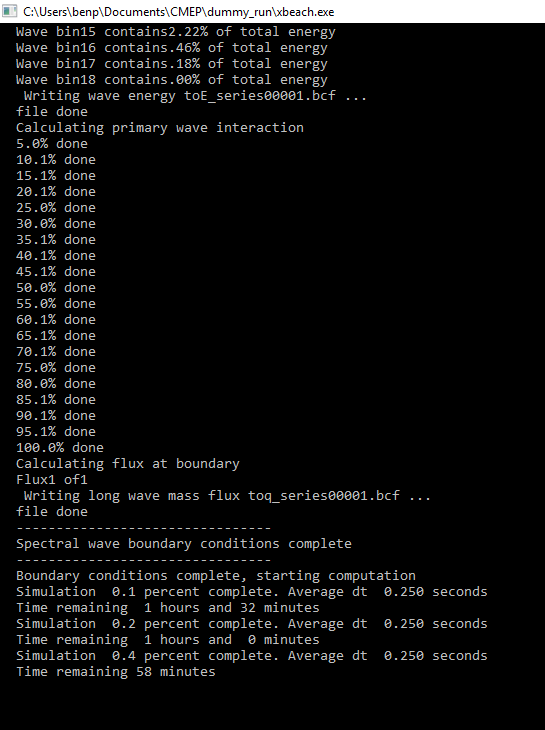
Open up XBlog.txt in a Text Editor since this records XBeach's progress, any errors etc. Here, you can double check that the correct files are being used. You can see for yourself just how many settings XBeach has, and all the things the model can represent! When the model is finished you can also see how long the simulation took.

Good working practice and tips

Have a seperate folder for each model run, this will prevent files being confused. E.g. if you have 3 different profiles or 3 different wave/water level conditions, have 3 seperate folders.
Start XBeach at low tide to allow time to 'spin-up' and stabilise, particularly when running with beach erosion enabled.

Reading and plotting XBeach output

Ideally we would output a single netCDF4 file containing all the XBeach output. However due to software requirements, we will output simple fortran binary files, which have the file extension ".dat". In this section, you will be provided with the following scripts:

plot_wave_runup.py : This script saves the wave run-up to a text file, allowing you to plot in whatever software you feel most comfortable with, whether it is Microsoft Excel, or (hopefully) Python! It also prints some basic exceedance statistics to screen.
plot_storm_profile.py: This script saves the initial and the end beach profiles to a text file, allowing you to plot the output.

Plotting wave run-up

Ensure that your working directory (folder path in top right hand side of Spyder screen) is set to the xbeach-model, since this contains the Python plotting scripts and the .dat files, and set the name of the file to save the time series to.

# -*- coding: utf-8 -*-
"""
Created on Fri Nov 23 10:27:15 2018
plot_wave_runup.py
@author: benp

This script will read XBeach binary files and plot a time series of wave runup.
It will also save the time series to a specified text file, allowing the user to 
plot it elsewhere.
"""

import matplotlib.pyplot as plt
import numpy as np
from cmep_xbeach import PlotWaveRunUp_Fortran
plt.rc('font',size=20)

#Set parameters below
OutputFile = 'wave_runup.txt' #File to save the time series of wave run-up to

### Please do not change anything below here ###
RunUp,Time = PlotWaveRunUp_Fortran(OutputFile)
plt.xlabel('Time (seconds)')
plt.ylabel('Wave Run-Up (m)')
plt.xlim([0,Time[-1]])
plt.plot(Time,RunUp,'k',linewidth=0.15)

Maximum wave run-up(m):  1.03
2% exceedance wave run-up (m):  0.59
5% exceedance wave run-up (m): 0.52
10% exceedance wave run-up (m): 0.46

Running the above scripts produces both a Python plot and a comma-delimited file of the time series of wave run-up. It also prints some basic statistics to the screen. This can now easily be plotted in Microsoft Excel by going to Data > From text and reading in the file

Plotting post-storm profiles

Ensure that your working directory (folder path in top right hand side of Spyder screen) is set to the xbeach-model, since this contains the Python plotting scripts and the .dat files, and set the name of the file to save the storm profiles to.:

X[Offshore],Initial Profile[Offshore], Final Profile[Offshore]

X[1],Initial Profile[1], Final Profile[1]

X[Land], Initial Profile[Land], Final Profile[Land]

# -*- coding: utf-8 -*-
"""
Created on Fri Nov 23 10:27:15 2018
plot_storm_profiles.py
@author: benp

This script will read the Fortran binary files and plot the initial and end bed profiles,
allowing the user to view the amount of erosion throughout the model run. It also saves
them to a user specified file
"""

import matplotlib.pyplot as plt
import numpy as np
from cmep_xbeach import PlotStormProfile_Fortran

OutputFile = 'model_profiles.txt' #File to save the initial and final beach profiles to.

### Please do not change anything below here ###
Data = PlotStormProfile_Fortran(OutputFile)
plt.plot(Data[:,0],Data[:,1],'k',label='Initial Profile') #plot and label graph
plt.plot(Data[:,0],Data[:,2],'r',label='Final Profile')
plt.xlabel('Cross-shore distance (m)')
plt.ylabel('Elevation (m)')

Summary

Hopefully you enjoyed the workshop and now you are confident in how to set-up and run a basic, one-dimensional XBeach model from both observational and modelled input data, and can use the model to predict wave run-up and cross-shore changes in a beach profile in your own applications. Please feel free to get in touch with me if you have any further questions, my email address can be found at the top of the page. Another great place to find help/advice or ask questions is the XBeach forum (https://oss.deltares.nl/web/xbeach/forum).